Viewing Results
Once we have run HypeSpace, we can then check in to see how the optimization performed. If you recall from previous tutorials, we specified a results_path within the hyperdrive function. This specified the path where we saved the results from the distributed run. Loading those results is as simple as
from my_optimization import objective
from hyperspace.kepler.data_utils import load_results


path = '/results_path'
results = load_results(path, sort=True)
Pointing load_results to the directory that we saved the HyperSpace results to returns a list of Scipy.OptimizeResults objects. By setting sort=True, we sort the results by the minimum found in ascending order. Note that we have imported the objective function here. This is because the Python pickles the reference to that namespace whenever it saves Scipy.OptimizeResults objects. Each element of this list of results contains all of the information gained through the optimization process for the respective distributed ranks. This includes the following:
- fun: the minimum found by the optimization
- func_vals: the function value found at each iteration of the optimization
- models: the specification of the surrogate model at each iteration
- random_state: the random seed
- space: the bounds of the search space for that particular rank
- specs: the specification for the Bayesian SMBO
- x: point found in the domain that returns the minimal fun value
- x_iters: the point in domain sampled at each iteration of the optimization
We can then visualize the course of the optimization with the following:
from hyperspace.kepler.plots import plot_convergence


best_result = results.pop(0)

_ = plot_convergence(results, best_result)
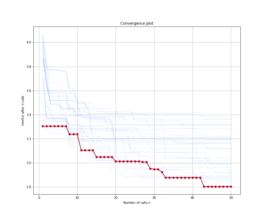
The above figure shows the convergence plot when optimizing five hyperparameters of our regression model from our Gradient Boosted Trees example. The traces show the optimization progress at each rank as we run 50 iterations of Bayesian SMBO in parallel. The red trace shows the best performing rank.
Note that the plot_convergence function can accept a list of HyperSpace results (results in this case), and it can accept a single rank’s result (best_results here). If we had many traces from a large scale run, it can sometimes be helpful to look at only a few of the traces at a time. Here is how we can look at the top five results from the above HyperSpace run:
_ = plot_convergence(results[0], results[1], results[2], results[3], best_result)
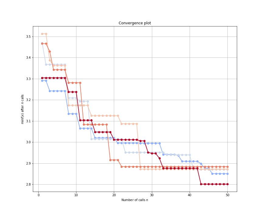
By examining the optimization traces, we could then decide to prune some of the search spaces in the future. Since machine learning is always an iterative process, understanding the behavior of our models over various hyperparameter search spaces can inform future model building.
We can also explore the effects of the hyperparameters within each of the search spaces. Since Scikit-Optimize [2] is integrated into HyperSpace, we can then explore the partial dependencies between hyperparameters. Originally proposed by Jerome H. Friedman, partial dependence plots were designed to visualize the effects of input variables for gradient boosted machines [1]. Here we can use them to understand the partial dependence of our objective function on each of the hyperparameters, holding all others constant, as well as all two-way interactions between hyperparameters, again holding all others constant.
from skopt.plots import plot_objective


_ = plot_objective(best_result)
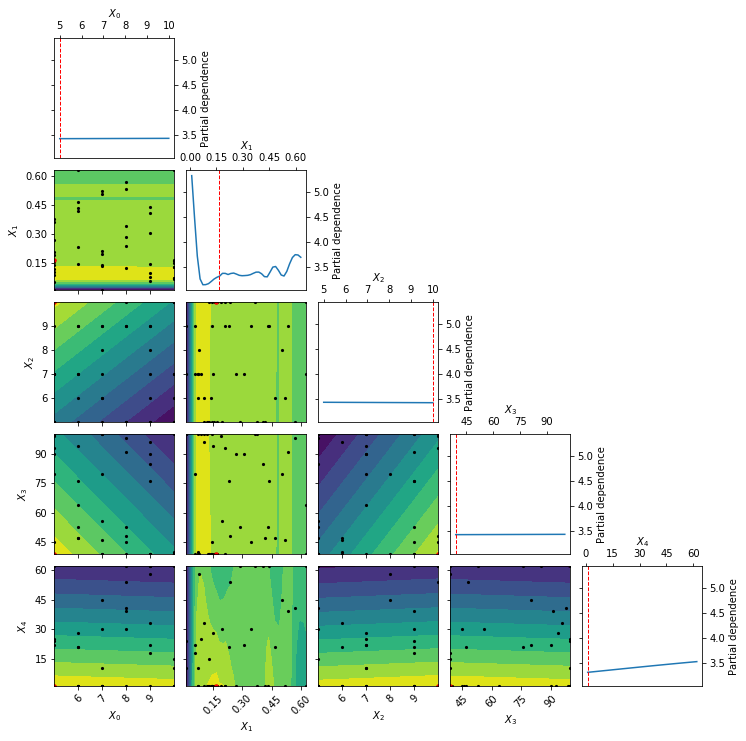
The above partial dependence plot shows how our objective function behaves at various settings of our model hyperparameters when considering the best hyperparameter subspace found by HyperSpace. Along the diagonal we have the effect of each hyperparameter, holding all other hyperparameters constant, on the five fold cross validation loss for our gradient boosted regressor. The dotted red line each of those subplots indicates the final setting of the hyperparameter. All off-diagonal plots show the two-way interactions for the hyperparameters, holding all other hyperparameters constant. The black points within these subplots show the points sampled along the two search dimensions. The red point in each of those subplots shows the final setting for the hyperparameters. The countours on the two-way interactions subplots show the loss landscape as viewed by our surrogate Gaussian process. Yellow contours indicate lower regions in the loss, whereas blue regions show higher loss values.
Note that the above partial dependence example shows the partial dependence of our hyperparameters within the best performing search space found by HyperSpace. We can also inspect these partial dependencies for all other search spaces used by HyperSpace. By doing so we can explore how a change in the bounds of the search space effects our optimization. We can therefore view where the models are performing well and where they are performing poorly. This is key to better understanding how our models behave. It is not only useful to find when our models perform well, knowing when the models will break down is equally important!
As we iterate through the model building process, it is helpful to visualize the outcomes of the optimization process. This allows us to inject our preferences and intuitions into the process so that we can better steer future directions.
References
| [1] | Jerome H. Friedman. Greedy function approximation: a gradient boosting machine. Ann. Statist., 29(5):1189–1232, 10 2001. URL: https://doi.org/10.1214/aos/1013203451, doi:10.1214/aos/1013203451. |
| [2] | Tim Head, MechCoder, Gilles Louppe, Iaroslav Shcherbatyi, fcharras, Zé Vinícius, cmmalone, Christopher Schröder, nel215, Nuno Campos, Todd Young, Stefano Cereda, Thomas Fan, rene-rex, Kejia (KJ) Shi, Justus Schwabedal, carlosdanielcsantos, Hvass-Labs, Mikhail Pak, SoManyUsernamesTaken, Fred Callaway, Loïc Estève, Lilian Besson, Mehdi Cherti, Karlson Pfannschmidt, Fabian Linzberger, Christophe Cauet, Anna Gut, Andreas Mueller, and Alexander Fabisch. Scikit-optimize/scikit-optimize: v0.5.2. March 2018. doi:10.5281/zenodo.1207017. |